


01 What Is a Pump Curve?
Every centrifugal pump has a personality. That personality is captured in a single graphical document supplied by the vendor before the pump ever ships to site: the pump performance curve.
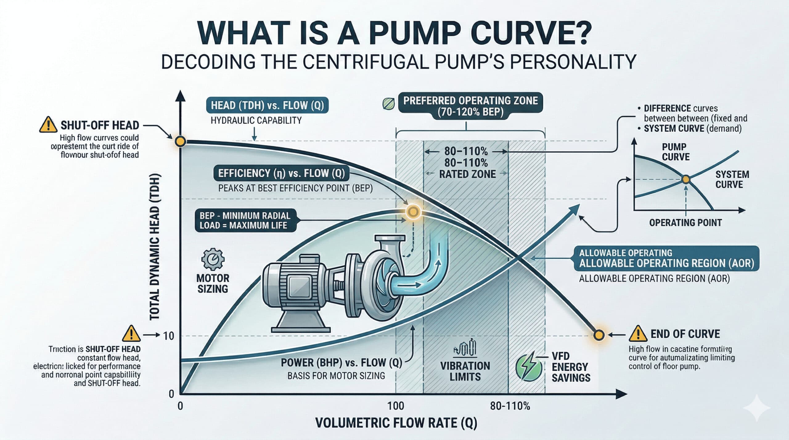
At its core, the pump curve is a plot of Total Dynamic Head (TDH) against volumetric flow rate (Q). But a complete performance chart overlays three distinct curves on the same axes:
Head delivered vs. flow rate. Defines the pump’s hydraulic capability. Always slopes downward from left to right.
Pump efficiency vs. flow rate. Bell-shaped curve that peaks at the Best Efficiency Point (BEP).
Brake Horsepower (shaft power) vs. flow rate. Rises continuously — the basis for motor sizing.
▲ All three performance curves plotted against % BEP flow. Hover to inspect regions. Preferred operating zone shaded in teal.
02 The Head–Flow (H–Q) Curve
The H–Q curve is the pump’s hydraulic signature. It answers a single question: for a given flow demand from the system, how much head will this pump deliver?
The relationship is governed by the energy exchange between the rotating impeller and the liquid. As the impeller spins, it imparts kinetic energy to the liquid. The volute casing then converts this kinetic energy into pressure head. The efficiency of this conversion depends critically on how well the liquid’s velocity triangles at the impeller vanes match the impeller geometry — and that match degrades as flow moves away from the design point.
The shape of the H–Q curve carries important information. A steep curve (large head change per unit flow change) gives good flow control sensitivity — a small change in system resistance produces a small change in flow. A flat curve delivers nearly constant flow across a wide range of system heads, which suits applications like boiler feed where stable flow matters more than stable head.
03 Why Does Head Drop with Flow?
The descending H–Q slope is not arbitrary — it is the result of six distinct loss mechanisms that grow as flow rate increases. Understanding each one transforms the pump curve from an abstract line into a physical story.
Loss Breakdown at High Flow
Relative magnitude at high flow (above BEP) · Source: Pump Performance Curve Prediction Methodology
04 Shut-Off Head: The Zero-Flow Condition
Follow the H–Q curve all the way to the left — to Q = 0 — and you arrive at the shut-off head. This is the maximum differential pressure the pump can develop, expressed as head, when no flow is moving through it.
At shut-off, the impeller rotates at full speed inside a sealed volume of liquid. All the impeller’s energy input manifests as pressure. No useful work is performed in terms of fluid transport — the energy is simply stored as static head at the discharge.
This is why minimum flow protection — typically a recirculation line with a minimum flow control valve — is mandated for all pumps handling liquids near their bubble point, and recommended for all centrifugal pumps in critical service.
Note that some end-suction centrifugal pump designs exhibit a characteristic known as a drooping H–Q curve near shut-off. Instead of the head rising monotonically as flow decreases, the head actually drops slightly before reaching the true shut-off value. This drooping behaviour, caused by volute friction losses rising steeply at very low flow, can create instability on flat system curves and must be flagged during pump selection for such applications.
05 The Efficiency Curve
The efficiency versus flow curve is the bell-shaped curve that every pump engineer has burned into memory. Its shape tells the story of how well the pump converts the mechanical power supplied by the shaft into useful hydraulic power delivered to the fluid.
Pump hydraulic efficiency is defined as:
Three Regions of the Efficiency Curve
Region 1 — Low Flow (Left of BEP): Efficiency is low because the impeller rotates at design speed but flow is restricted. The liquid cannot follow the intended path through the vane passages. A portion of the discharge flow recirculates back toward the impeller eye — a phenomenon called suction recirculation. This recirculation generates intense local turbulence, heats the liquid, and creates localised low-pressure zones that can trigger cavitation even when the system NPSH appears adequate. Energy is consumed by the motor and converted to heat rather than useful head.
Region 2 — Rising Efficiency (Approaching BEP): As flow increases, the velocity triangles at the impeller inlet progressively align with the vane angles. Recirculation diminishes. The liquid moves along the designed flow path, and the energy conversion from shaft power to hydraulic head improves steadily. Efficiency climbs.
Region 3 — Falling Efficiency (Beyond BEP): Past the BEP flow, liquid velocities inside the pump rise rapidly. Friction losses on the impeller vane surfaces and the volute scale approximately with velocity squared. Flow separation from the vane trailing edges creates additional turbulence. The efficiency curve turns over and descends, even though more liquid is being moved per unit time.
06 Best Efficiency Point (BEP) — Decoded
The BEP is the single most important point on the pump curve. It is not merely a performance metric — it is a mechanical reliability indicator.
Pump selection closer to the BEP yields a more efficient pump with the least amount of vibration and radial forces acting on the shaft. In the case of single-volute pumps, operating away from the BEP causes the shaft to deflect, with bearings and seals rubbing against casing components. The fluid flow angle into the impeller also fails to align with impeller speeds and vane angles, causing suction recirculation, fluid stall, and cavitation.
What Happens Mechanically at BEP
At BEP, the hydraulic design condition is exactly met. The relative velocity of the liquid at the impeller inlet is aligned with the leading-edge vane angle — no incidence loss occurs. The flow exits the impeller with the designed exit angle. The volute collects the discharge uniformly around its perimeter, creating a balanced radial pressure distribution. This hydraulic balance means:
| Parameter | At BEP | Away from BEP |
|---|---|---|
| Radial Shaft Load | Minimum — hydraulically balanced | Elevated — asymmetric volute pressure |
| Bearing Life | Maximum (L10 life achieved) | Reduced — elevated radial load |
| Mechanical Seal Life | Maximum (low shaft deflection) | Reduced — shaft vibration & deflection |
| Vibration Level | Minimum | Elevated — risk of resonance |
| Temperature Rise | Minimum | Significant (especially at low flow) |
| Cavitation Risk | Lowest NPSHr | Rises steeply away from BEP |
07 The Power (BHP) Curve
The Brake Horsepower curve describes the shaft power that must be delivered to the pump by its driver at every operating point. For most centrifugal pumps, this curve rises continuously from left to right — a characteristic with significant practical implications for motor sizing and electrical protection.
Power at Zero Flow (Shut-Off)
Even with the discharge valve fully closed and zero flow moving through the pump, the motor continues to draw power. The impeller rotates inside the liquid, overcoming viscous drag, bearing friction, and mechanical seal friction. This zero-flow power draw is real, measurable, and must be accounted for in motor protection relay settings.
Motor Sizing Rule
A common engineering error is to size the motor based on the design-point power consumption. This is wrong. The motor must be sized for the maximum power point on the pump curve, which for most centrifugal pumps occurs at or near the end of the curve — maximum flow, minimum head.
End of the Curve
The rightmost point of the H–Q curve, where head reaches its minimum and flow its maximum, is called the End of Curve. At this point, system resistance is at its absolute minimum (all control valves wide open, no artificial restriction). The pump delivers maximum possible flow but at the lowest possible efficiency.
Operating at the end of the curve also means the Net Positive Suction Head Required (NPSHr) is at its highest value — increasing cavitation risk significantly if the suction system has limited available NPSH.
08 API 610 Operating Zones — What the Standard Says
API 610 (Centrifugal Pumps for Petroleum, Petrochemical and Natural Gas Industries) defines three distinct operating regions relative to BEP. These are not arbitrary — they are derived from mechanical reliability data linking operating position to bearing, seal, and impeller failure rates.
| Zone | API 610 Definition | Flow Range | Primary Failure Mode | Recommended Action |
|---|---|---|---|---|
| DANGER | Below Min. Stable Continuous Flow (MSCF) | ≪ 70% BEP | Suction recirculation, thermal damage | Minimum flow recirculation line mandatory |
| ALLOWABLE | Allowable Operating Region (AOR) | Set by manufacturer | Elevated vibration, reduced life | Avoid continuous operation; acceptable for transients |
| PREFERRED | Preferred Operating Region (POR) | 70 – 120% BEP | None — within design intent | Target for continuous operation |
| RATED | Rated Region (Min/Max Operable) | 80 – 110% BEP | None — optimal zone | Design point should fall here per API 610 |
09 Affinity Laws & VFD Control
The H–Q curve described so far applies to a pump running at a fixed rotational speed. When a Variable Frequency Drive (VFD) is added, the pump can operate at multiple speeds — and for each speed, there is a distinct H–Q curve. The relationship between speed and performance is governed by the Affinity Laws (also called Fan Laws, since liquids behave as incompressible fluids).
When VFDs Are Not the Answer
VFDs are often proposed as a universal solution, but there are important cases where they are inappropriate or even harmful:
| Scenario | VFD Suitability | Reason |
|---|---|---|
| High static head systems (e.g. boiler feed) | ⚠️ Limited | Low speed may not generate enough head to overcome static head — pump stalls |
| Improperly selected pump | ❌ Inappropriate | VFD cannot compensate for wrong pump selection — buy the right pump |
| Variable process demand | ✅ Ideal | Speed follows demand — eliminates control valve throttling losses |
| Constant flow service | ⚡ Limited benefit | Fixed speed drive more cost-effective; VFD adds cost without proportional gain |
10 The Pump Curve as a Diagnostic Tool
The pump performance curve is not only a design and selection tool — it is a living reference document for field diagnostics. An engineer who knows how to read the curve and compare it to live operating data can identify most pump problems before they escalate to failure.
Field Diagnostic Matrix
| Observed Symptom | Curve Reading | Likely Cause |
|---|---|---|
| Flow below design, head normal | Operating left of design point | Increased system resistance; partially closed valve; control valve issue |
| Flow above design, head low | Operating right of design point | System resistance lower than design; check valve failed open; bypass open |
| Head below OEM curve at same flow | Curve has shifted downward | Impeller wear; increased internal clearances; impeller erosion/corrosion |
| Excessive vibration + noise | Operating far from BEP | Suction or discharge recirculation; cavitation; resonance |
| High motor current | Operating near end of curve | System resistance lower than expected; pump overloading motor |
| Rapid seal failure | Operating left of 70% BEP | Shaft deflection from hydraulic imbalance; recirculation-induced vibration |
In brownfield revamp projects, where existing pumps are re-evaluated for new process conditions without original equipment manufacturer (OEM) data, predicting the pump curve from first principles using impeller geometry and the methodology described in engineering literature allows engineers to assess whether the pump can deliver the required head — and identify whether impeller trimming, speed change, or full replacement is the appropriate solution.
∑ Summary
The pump performance curve is three curves in one. Each speaks a different language:
Head decreases as flow increases. Set by impeller geometry and speed. Independent of system. Shut-off head at zero flow. Motor overload risk at end of curve.
Bell-shaped curve peaking at BEP. Operation outside 70–120% BEP accelerates bearing and seal failure. BEP = minimum radial load = maximum mechanical life.
Rises continuously with flow. Motor must be sized for maximum power point — not design point. Power scales with speed cubed — the VFD energy saving case.
if you want to write an article on the website, please contact us by this mail id: contact@worldofinstrumentation.com
If you like this article, and if you want to know about Next-Generation Pressure Measurement: Yokogawa EJX S Series vs. Emerson Rosemount 4051S Check out my previous article.
And you can also follow our LinkedIn group which is specially made for sharing information related to Industrial Automation and Instrumentation.

